Ventricle WGCNA
Last updated: 2019-12-02
Checks: 6 1
Knit directory: bentsen-rausch-2019/
This reproducible R Markdown analysis was created with workflowr (version 1.4.0). The Checks tab describes the reproducibility checks that were applied when the results were created. The Past versions tab lists the development history.
Great! Since the R Markdown file has been committed to the Git repository, you know the exact version of the code that produced these results.
The global environment had objects present when the code in the R Markdown file was run. These objects can affect the analysis in your R Markdown file in unknown ways. For reproduciblity it’s best to always run the code in an empty environment. Use wflow_publish or wflow_build to ensure that the code is always run in an empty environment.
The following objects were defined in the global environment when these results were created:
| Name | Class | Size |
|---|---|---|
| data | environment | 56 bytes |
| env | environment | 56 bytes |
The command set.seed(20191021) was run prior to running the code in the R Markdown file. Setting a seed ensures that any results that rely on randomness, e.g. subsampling or permutations, are reproducible.
Great job! Recording the operating system, R version, and package versions is critical for reproducibility.
Nice! There were no cached chunks for this analysis, so you can be confident that you successfully produced the results during this run.
Great job! Using relative paths to the files within your workflowr project makes it easier to run your code on other machines.
Great! You are using Git for version control. Tracking code development and connecting the code version to the results is critical for reproducibility. The version displayed above was the version of the Git repository at the time these results were generated.
Note that you need to be careful to ensure that all relevant files for the analysis have been committed to Git prior to generating the results (you can use wflow_publish or wflow_git_commit). workflowr only checks the R Markdown file, but you know if there are other scripts or data files that it depends on. Below is the status of the Git repository when the results were generated:
Ignored files:
    Ignored:    .Rproj.user/
    Ignored:    test_files/

Untracked files:
    Untracked:  analysis/figure_6.Rmd
    Untracked:  analysis/figure_7.Rmd
    Untracked:  analysis/supp1.Rmd
    Untracked:  code/sc_functions.R
    Untracked:  data/bulk/
    Untracked:  data/fgf_filtered_nuclei.RDS
    Untracked:  data/figures/
    Untracked:  data/filtglia.RDS
    Untracked:  data/glia/
    Untracked:  data/lps1.txt
    Untracked:  data/mcao1.txt
    Untracked:  data/mcao_d3.txt
    Untracked:  data/mcaod7.txt
    Untracked:  data/mouse_data/
    Untracked:  data/neur_astro_induce.xlsx
    Untracked:  data/neuron/
    Untracked:  data/synaptic_activity_induced.xlsx
    Untracked:  output/agrp_pcgenes.csv
    Untracked:  output/all_wc_markers.csv
    Untracked:  output/allglia_wgcna_genemodules.csv
    Untracked:  output/bulk/
    Untracked:  output/fig.RData
    Untracked:  output/fig4_part2.RData
    Untracked:  output/glia/
    Untracked:  output/glial_markergenes.csv
    Untracked:  output/integrated_all_markergenes.csv
    Untracked:  output/integrated_neuronmarkers.csv
    Untracked:  output/neuron/

Unstaged changes:
    Modified:   analysis/10_wc_pseudobulk.Rmd
    Modified:   analysis/11_wc_astro_wgcna.Rmd
    Modified:   analysis/13_olig_pseudotime.Rmd
    Modified:   analysis/15_tany_wgcna_pseudo.Rmd
    Modified:   analysis/6_glial_dge.Rmd
    Modified:   analysis/9_wc_processing.Rmd
    Modified:   analysis/figure_1.Rmd
    Modified:   analysis/index.Rmd
Note that any generated files, e.g. HTML, png, CSS, etc., are not included in this status report because it is ok for generated content to have uncommitted changes.
These are the previous versions of the R Markdown and HTML files. If you’ve configured a remote Git repository (see ?wflow_git_remote), click on the hyperlinks in the table below to view them.
| File | Version | Author | Date | Message |
|---|---|---|---|---|
| Rmd | e803f0d | Full Name | 2019-12-02 | wflow_publish(c(“analysis/8_astro_wgcna.Rmd”, |
| html | f4dd96b | Full Name | 2019-10-29 | Build site. |
| Rmd | 650ab6b | Full Name | 2019-10-28 | wflow_git_commit(all = T) |
| html | 9cf1e45 | Full Name | 2019-10-28 | Build site. |
Load Libraries
library(Seurat)
library(WGCNA)
library(cluster)
library(parallelDist)
library(ggsci)
library(emmeans)
library(lme4)
library(ggbeeswarm)
library(genefilter)
library(tidyverse)
library(reshape2)
library(igraph)
library(gProfileR)
library(ggpubr)
library(here)
library(ggforce)
library(tidygraph)
library(igraph)
library(ggraph)
library(cowplot)
library(future)
plan("multiprocess", workers=40)
options(future.globals.maxSize = 4000 * 1024^2)
Extract Cells for WGCNA
Calculate softpower
enableWGCNAThreads()Allowing parallel execution with up to 79 working processes.datExpr<-as.matrix(t(ventric[["SCT"]]@scale.data[ventric[["SCT"]]@var.features,]))
gsg = goodSamplesGenes(datExpr, verbose = 3); Flagging genes and samples with too many missing values...
..step 1powers = c(c(1:10), seq(from = 12, to=40, by=2))
sft=pickSoftThreshold(datExpr,dataIsExpr = TRUE, powerVector = powers, corOptions = list(use = 'p'),
networkType = "signed") Power SFT.R.sq slope truncated.R.sq mean.k. median.k. max.k.
1 1 0.186 -56.60 0.593 2.50e+03 2.50e+03 2570.000
2 2 0.536 -45.50 0.561 1.26e+03 1.25e+03 1350.000
3 3 0.924 -36.60 0.906 6.32e+02 6.27e+02 722.000
4 4 0.958 -24.60 0.975 3.18e+02 3.15e+02 398.000
5 5 0.950 -16.50 0.970 1.61e+02 1.58e+02 228.000
6 6 0.945 -11.60 0.971 8.18e+01 7.94e+01 135.000
7 7 0.945 -8.70 0.964 4.17e+01 4.00e+01 84.200
8 8 0.948 -6.70 0.961 2.14e+01 2.01e+01 54.800
9 9 0.964 -5.33 0.970 1.10e+01 1.01e+01 37.200
10 10 0.962 -4.40 0.964 5.75e+00 5.12e+00 26.200
11 12 0.981 -3.17 0.979 1.62e+00 1.31e+00 14.400
12 14 0.983 -2.48 0.978 4.93e-01 3.35e-01 8.650
13 16 0.965 -2.09 0.962 1.67e-01 8.65e-02 5.510
14 18 0.966 -1.79 0.966 6.57e-02 2.24e-02 3.650
15 20 0.947 -1.62 0.949 3.01e-02 5.85e-03 2.490
16 22 0.396 -2.00 0.345 1.57e-02 1.54e-03 1.730
17 24 0.389 -1.84 0.343 9.11e-03 4.09e-04 1.220
18 26 0.381 -1.74 0.327 5.67e-03 1.09e-04 0.873
19 28 0.960 -1.24 0.952 3.71e-03 2.95e-05 0.632
20 30 0.942 -1.21 0.927 2.53e-03 8.08e-06 0.465
21 32 0.956 -1.18 0.944 1.79e-03 2.25e-06 0.390
22 34 0.336 -1.82 0.232 1.29e-03 6.33e-07 0.329
23 36 0.981 -1.14 0.976 9.62e-04 1.80e-07 0.278
24 38 0.349 -1.75 0.252 7.31e-04 5.20e-08 0.235
25 40 0.353 -1.72 0.242 5.67e-04 1.53e-08 0.200cex1=0.9
plot(sft$fitIndices[,1], -sign(sft$fitIndices[,3])*sft$fitIndices[,2],xlab="Soft Threshold (power)",ylab="Scale Free Topology Model Fit, signed R^2",type="n", main = paste("Scale independence"))
text(sft$fitIndices[,1], -sign(sft$fitIndices[,3])*sft$fitIndices[,2],labels=powers ,cex=cex1,col="red")
abline(h=0.80,col="red")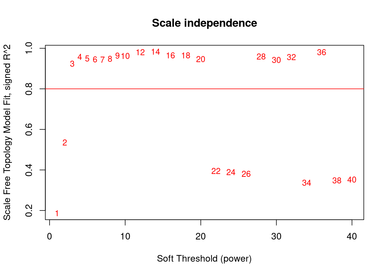
| Version | Author | Date |
|---|---|---|
| 9cf1e45 | Full Name | 2019-10-28 |
#Mean Connectivity Plot
plot(sft$fitIndices[,1], sft$fitIndices[,5],xlab="Soft Threshold (power)",ylab="Mean Connectivity", type="n",main = paste("Mean connectivity"))
text(sft$fitIndices[,1], sft$fitIndices[,5], labels=powers, cex=cex1,col="red")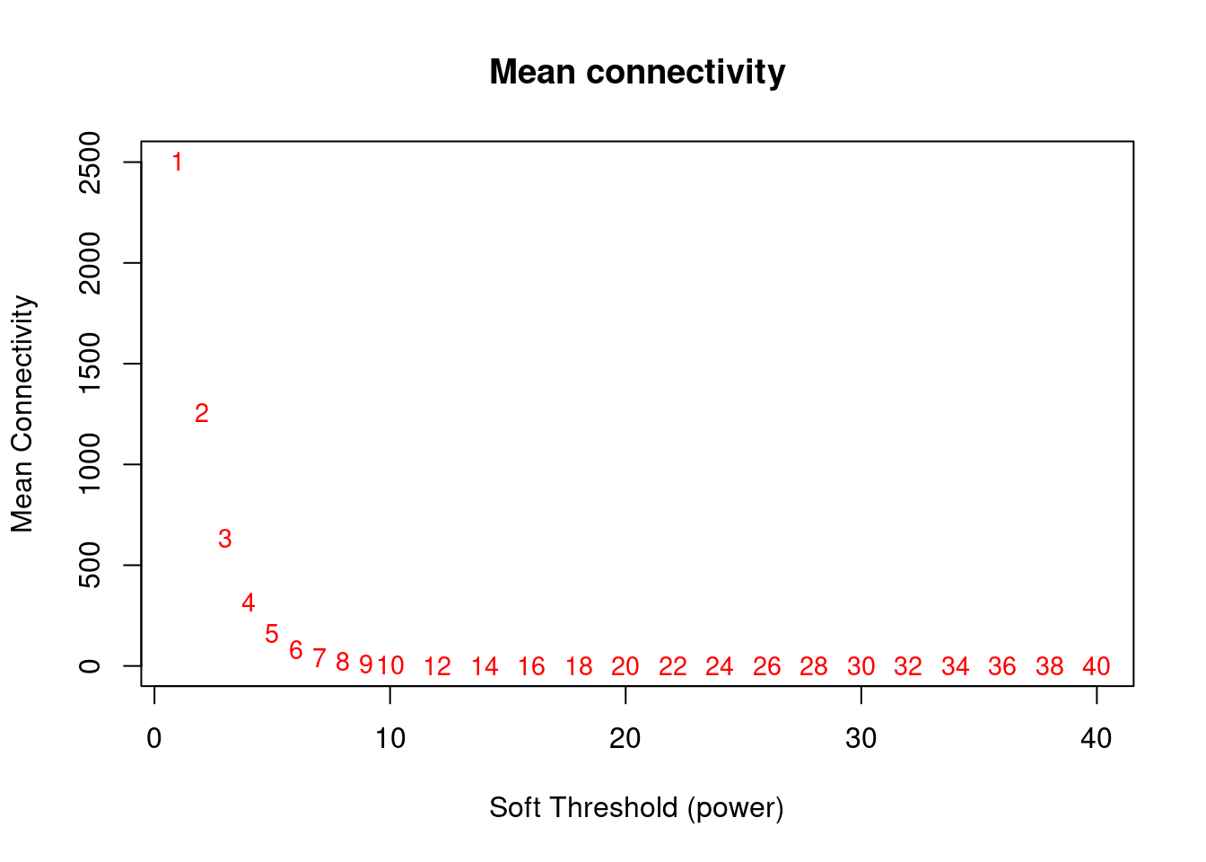
| Version | Author | Date |
|---|---|---|
| 9cf1e45 | Full Name | 2019-10-28 |
Generate TOM
softPower = 3
SubGeneNames<-colnames(datExpr)
adj= adjacency(datExpr, type = "signed", power = softPower)
diag(adj)<-0
TOM=TOMsimilarityFromExpr(datExpr, networkType = "signed", TOMType = "signed", power = softPower, maxPOutliers = 0.05)
TOM calculation: adjacency..
..will use 79 parallel threads.
Fraction of slow calculations: 0.000000
..connectivity..
..matrix multiplication (system BLAS)..
..normalization..
..done.colnames(TOM) = rownames(TOM) = SubGeneNames
dissTOM=1-TOM
geneTree = hclust(as.dist(dissTOM),method="average") #use complete for method rather than average (gives better results)
plot(geneTree,xlab="",sub="",cex=.5,main="Gene clustering",hang=.001)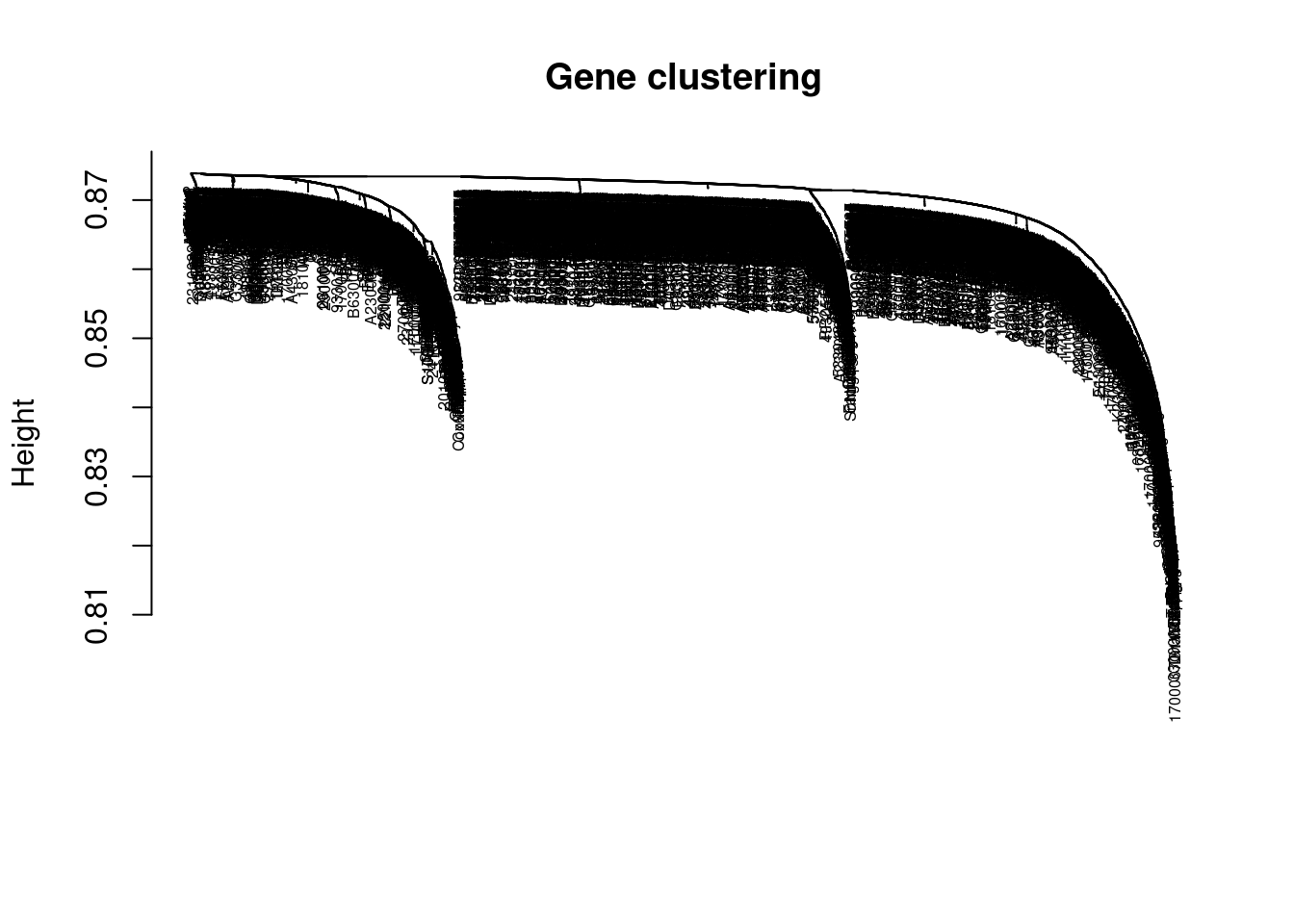
| Version | Author | Date |
|---|---|---|
| 9cf1e45 | Full Name | 2019-10-28 |
Identify Modules
minModuleSize = 15
x = 4
dynamicMods = cutreeDynamic(dendro = geneTree, distM = as.matrix(dissTOM),
                            method="hybrid", pamStage = F, deepSplit = x,
                            minClusterSize = minModuleSize)
..cutHeight not given, setting it to 0.874 ===> 99% of the (truncated) height range in dendro.
..done.dynamicColors = labels2colors(dynamicMods) #label each module with a unique color
plotDendroAndColors(geneTree, dynamicColors, "Dynamic Tree Cut",
dendroLabels = FALSE, hang = 0.03, addGuide = TRUE, guideHang = 0.05,
main = "Gene dendrogram and module colors") #plot the modules with colors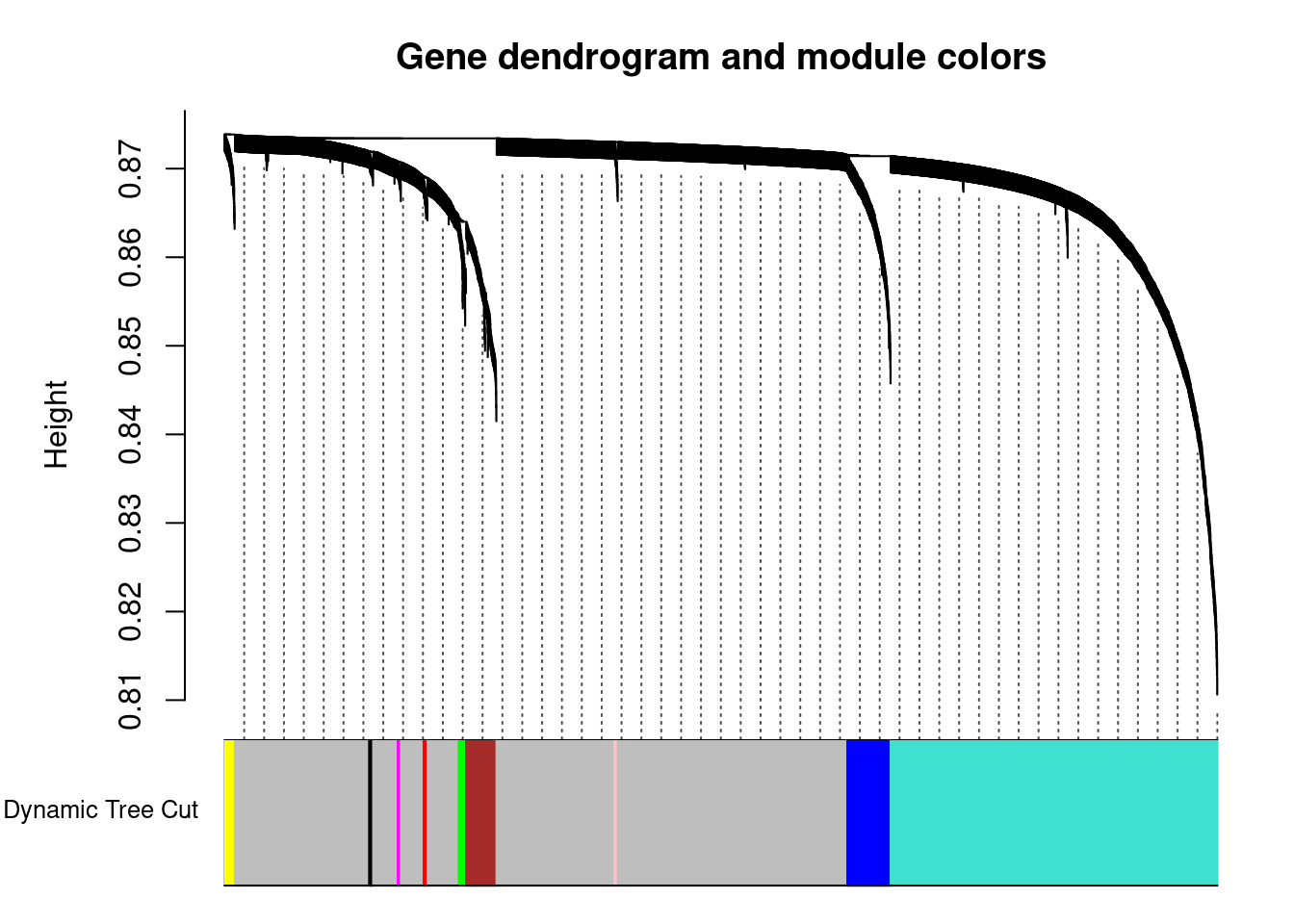
| Version | Author | Date |
|---|---|---|
| 9cf1e45 | Full Name | 2019-10-28 |
Calculate Eigengenes and Merge Close Modules
MEs = moduleEigengenes(datExpr, dynamicColors)$eigengenes
ME1<-MEs
row.names(ME1)<-row.names(datExpr)
MEDiss = 1-cor(MEs);
METree = hclust(as.dist(MEDiss), method = "average");
plot(METree, main = "Clustering of module eigengenes",xlab = "", sub = "")
MEDissThres = 0.2
abline(h=MEDissThres, col = "red")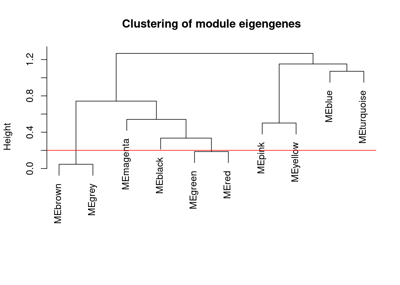
| Version | Author | Date |
|---|---|---|
| 9cf1e45 | Full Name | 2019-10-28 |
Merge modules
merge = mergeCloseModules(datExpr, dynamicColors, cutHeight = MEDissThres, verbose = 3) mergeCloseModules: Merging modules whose distance is less than 0.2
multiSetMEs: Calculating module MEs.
Working on set 1 ...
moduleEigengenes: Calculating 10 module eigengenes in given set.
multiSetMEs: Calculating module MEs.
Working on set 1 ...
moduleEigengenes: Calculating 9 module eigengenes in given set.
Calculating new MEs...
multiSetMEs: Calculating module MEs.
Working on set 1 ...
moduleEigengenes: Calculating 9 module eigengenes in given set.mergedColors = merge$colors
mergedMEs = merge$newMEs
moduleColors = mergedColors
MEs = mergedMEs
modulekME = signedKME(datExpr,MEs)Plot merged modules
plotDendroAndColors(geneTree, cbind(dynamicColors, mergedColors),
c("Dynamic Tree Cut", "Merged dynamic"),
dendroLabels = FALSE, hang = 0.03,
addGuide = TRUE, guideHang = 0.05)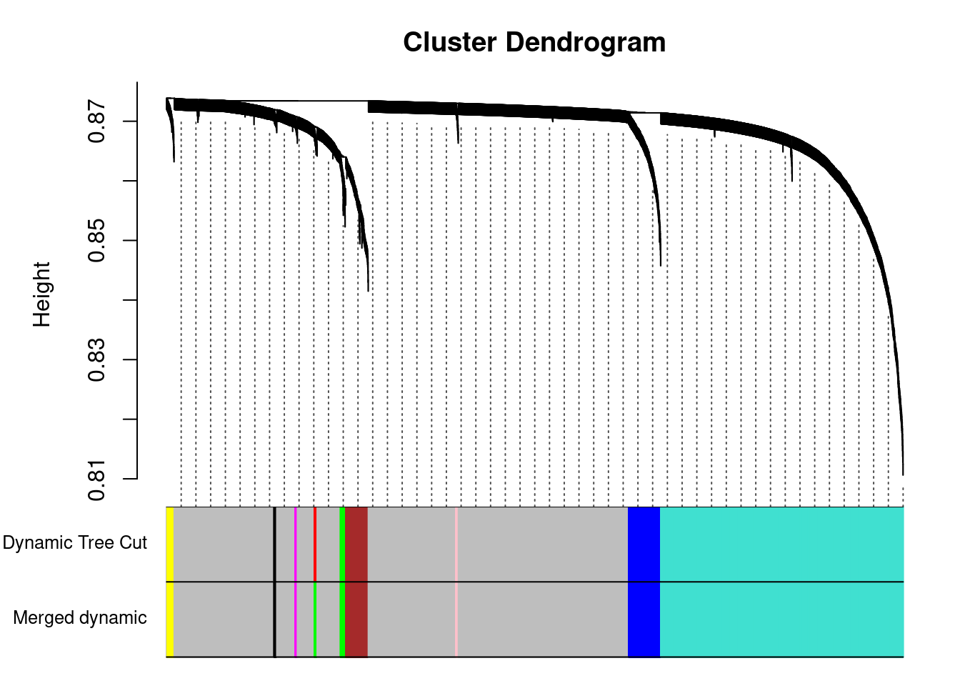
| Version | Author | Date |
|---|---|---|
| 9cf1e45 | Full Name | 2019-10-28 |
moduleColors = mergedColors
MEs = mergedMEs
modulekME = signedKME(datExpr,MEs)
Generate function to look up genes in each network
modules<-MEs
c_modules<-data.frame(moduleColors)
row.names(c_modules)<-colnames(datExpr)
module.list.set1<-substring(colnames(modules),3)
index.set1<-0
Network=list()
for (i in 1:length(module.list.set1)){index.set1<-which(c_modules==module.list.set1[i])
Network[[i]]<-row.names(c_modules)[index.set1]}
names(Network)<-module.list.set1
lookup<-function(gene,network){return(network[names(network)[grep(gene,network)]])}
Filter metadata table and correlate with eigengenes
nGenes = ncol(datExpr)
nSamples = nrow(datExpr)
MEs = orderMEs(MEs)
ventric$group<-paste0(ventric$trt,"_",ventric$day)
var<-model.matrix(~0+ventric$group)
moduleTraitCor <- cor(MEs, var, use="p")
moduleTraitPvalue = corPvalueStudent(moduleTraitCor, nSamples)
cor<-melt(moduleTraitCor)
ggplot(cor, aes(Var2, Var1)) + geom_tile(aes(fill = value),
     colour = "white") + scale_fill_gradient2(midpoint = 0, low = "blue", mid = "white",
                            high = "red", space = "Lab", name="Correlation \nStrength") +
  theme(axis.text.x = element_text(angle = 45, hjust = 1)) + xlab("Treatment") + ylab(NULL)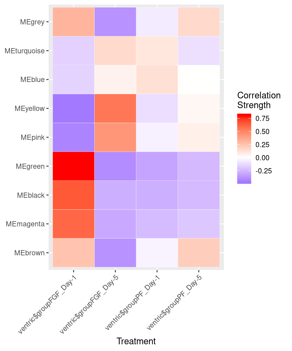
| Version | Author | Date |
|---|---|---|
| 9cf1e45 | Full Name | 2019-10-28 |
Get hubgenes in order
hubgenes<-lapply(seq_len(length(Network)), function(x) {
  dat<-modulekME[Network[[x]],]
  dat<-dat[order(-dat[paste0("kME",names(Network)[x])]),]
  gene<-rownames(dat)
  return(gene)
})

names(hubgenes)<-names(Network)
d <- unlist(hubgenes)
d <- data.frame(gene = d,
           vec = names(d))
write_csv(d, path=here("output/glia/wgcna/allglia_wgcna_genemodules_nokme.csv"))
Build linear models for differential expression
MEs %>% select(-MEgrey) -> MEs
data<-data.frame(MEs, day=ventric$day, trt=ventric$trt,
                 sample=as.factor(ventric$sample), group=ventric$group,
                 batch=ventric$batch, celltype=Idents(ventric),
                 groupall=paste0(Idents(ventric), ventric$group))

# loop through modules and perform linear regression
mod<-lapply(colnames(MEs), function(me) {
  # interaction between treatmet group and cell type
  # random effect for batch
  # random effect for sample
  mod<-lmer(MEs[[me]] ~ group*celltype + (1|batch) + (1|sample), data=data)
  # use emmeans to test pariwaise differences
  pairwise<-emmeans(mod, pairwise ~ group|celltype)
  plot<-data.frame(plot(pairwise, plotIt=F)$data)
  sig<-as.data.frame(pairwise$contrasts)
  sig%>%separate(contrast, c("start", "end"), sep = " - ") -> sig
  yvals<-unlist(lapply(unique(sig$celltype), function(x) {
    x<-as.character(x)
    y<-data[data$celltype==x,]
    z<-max(as.numeric(y[[me]]))
    names(z)<-x
    return(z)
  }))
  sig$yvals<-yvals[match(sig$celltype, names(yvals))]
  sig$yvals[duplicated(sig$yvals)]<-sig$yvals[duplicated(sig$yvals)]+.004
  sig$yvals[duplicated(sig$yvals)]<-sig$yvals[duplicated(sig$yvals)]+.004
  sig$yvals[duplicated(sig$yvals)]<-sig$yvals[duplicated(sig$yvals)]+.004
  return(sig)
})
Warning in checkConv(attr(opt, "derivs"), opt$par, ctrl =
control$checkConv, : Model failed to converge with max|grad| = 0.00359644
(tol = 0.002, component 1)names(mod) <- colnames(MEs)
sig <- bind_rows(mod, .id="id")
sig$symbol <- sig$p.value
# set ranges for significance markings
sig$symbol[findInterval(sig$symbol, c(0.1,2)) == 1L] <-NA
sig$symbol[findInterval(sig$symbol, c(0.01,0.1)) == 1L] <- "*"
sig$symbol[findInterval(sig$symbol, c(0.001,0.01)) == 1L] <- "**"Warning in findInterval(sig$symbol, c(0.001, 0.01)): NAs introduced by
coercionsig$symbol[findInterval(sig$symbol, c(1e-200,0.001)) == 1L] <- "***" Warning in findInterval(sig$symbol, c(1e-200, 0.001)): NAs introduced by
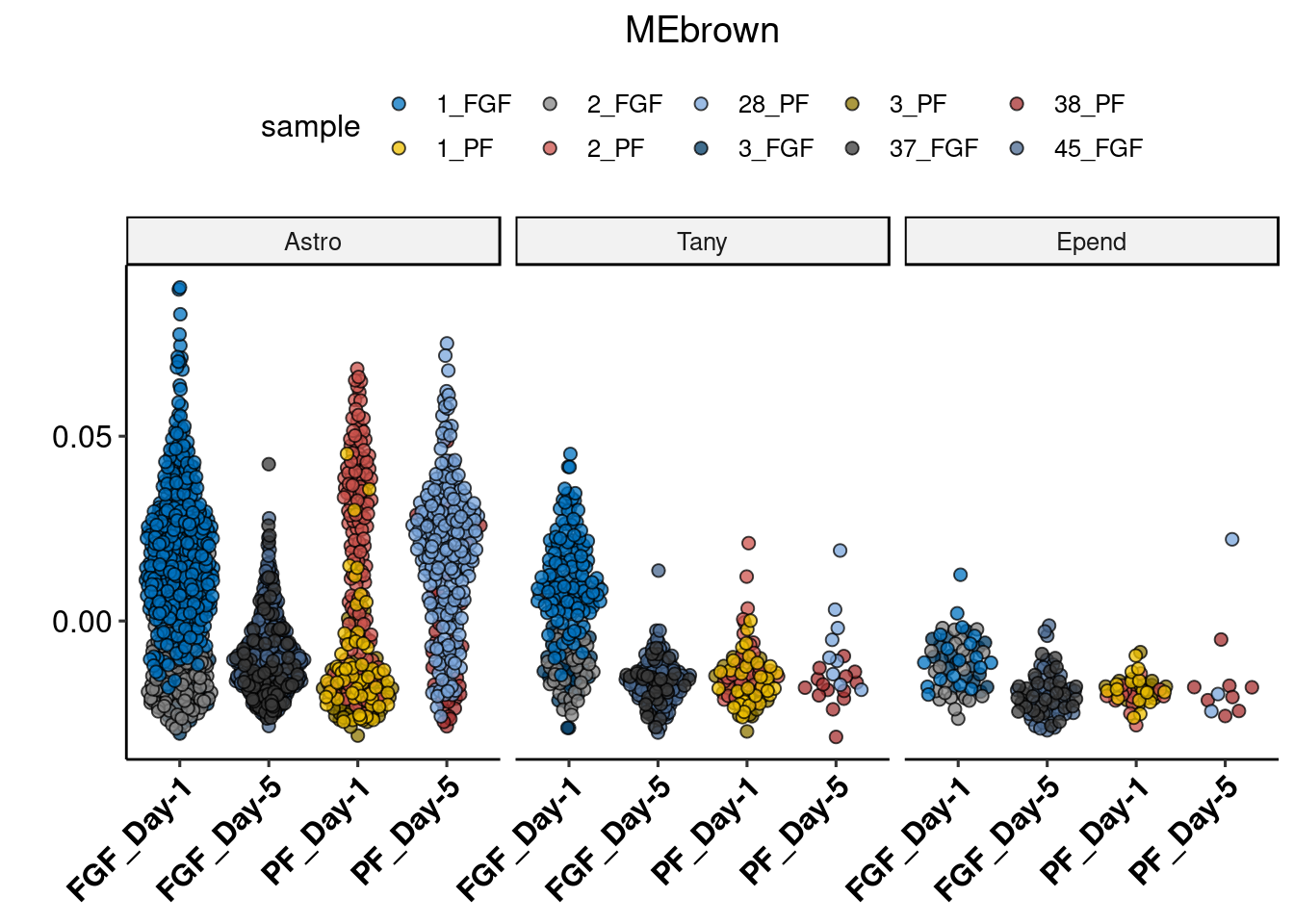
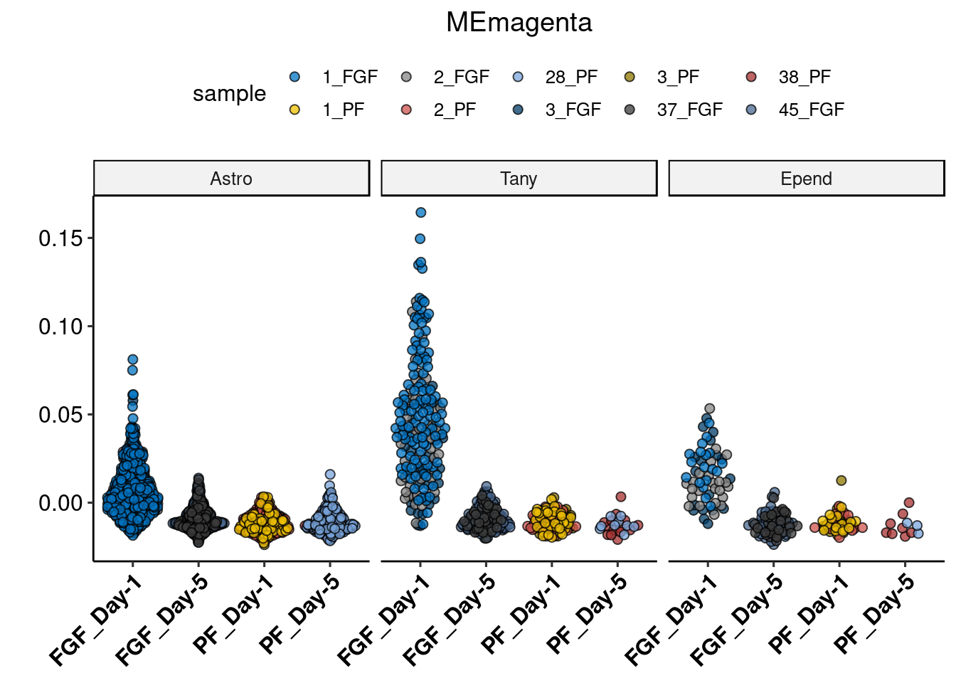
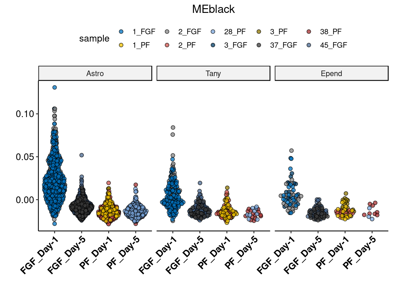
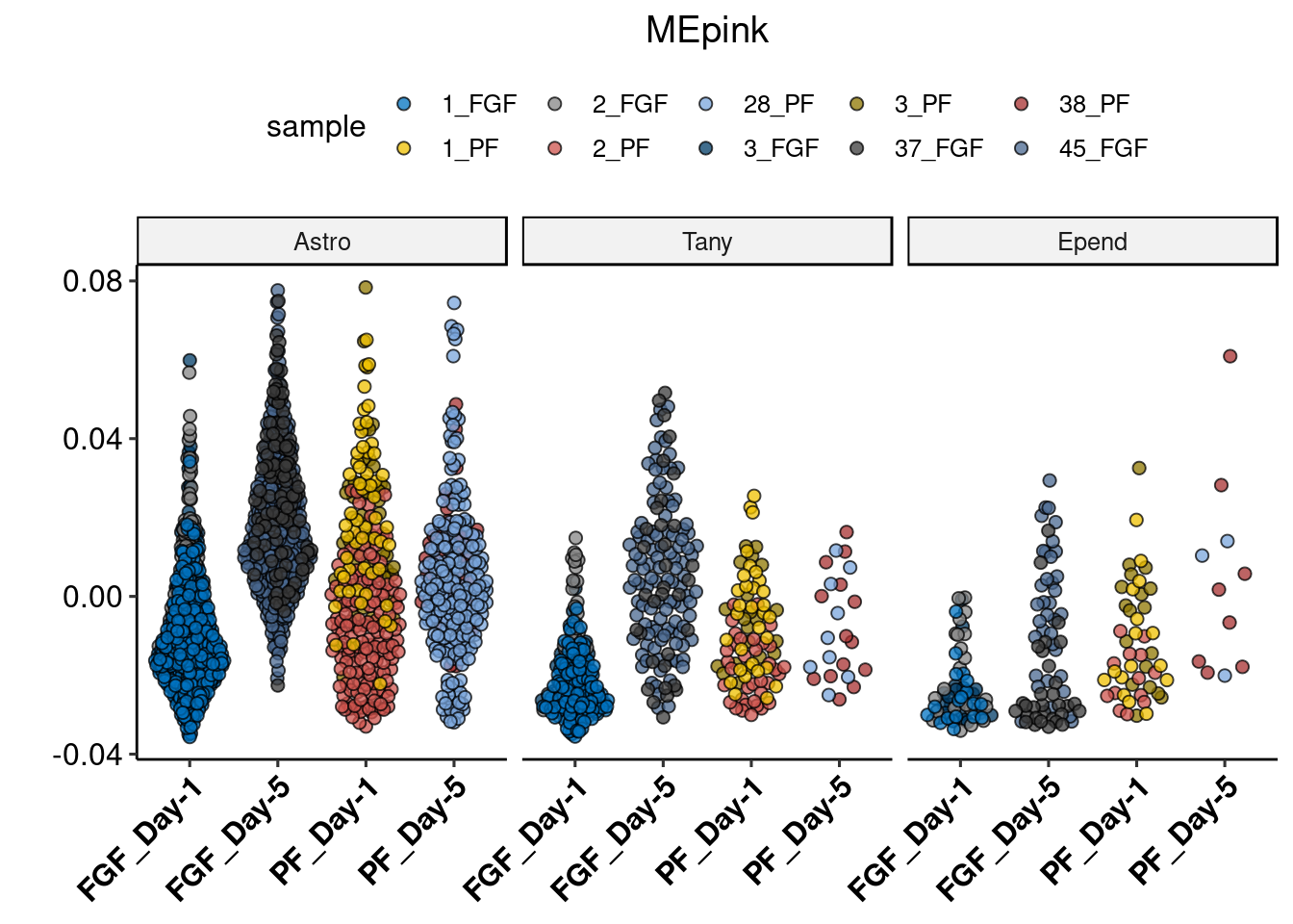
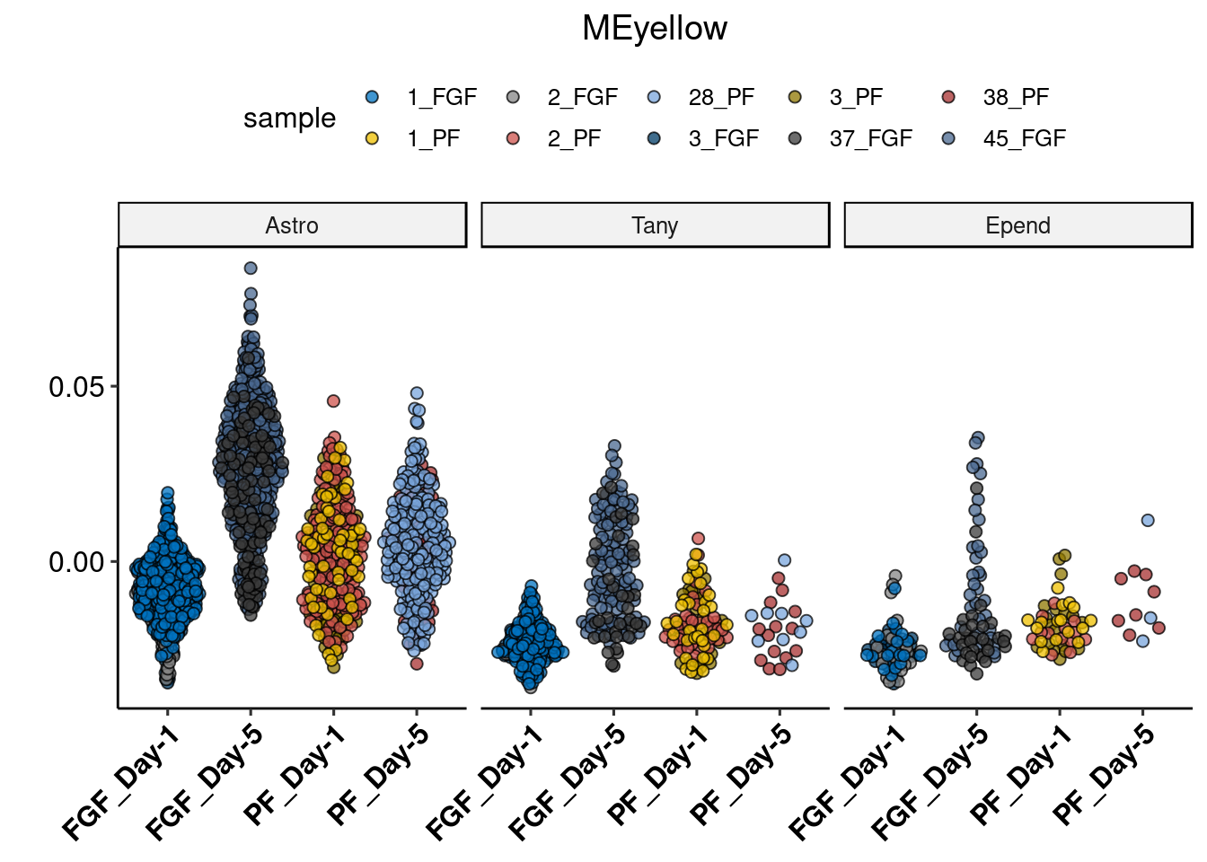
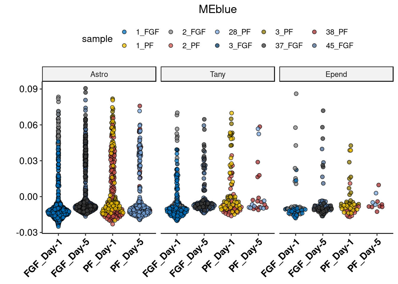
coerciondata <- melt(data, id.vars = c("day","trt","sample","group","batch","celltype","groupall"))
lapply(unique(data$variable), function(x) {
tryCatch({
print(ggplot(data=data[data$variable==x,], aes(x=group, y=as.numeric(value))) +
geom_quasirandom(aes(fill=sample), shape=21, size=2, alpha=.75) +
scale_fill_manual(values=pal_jco()(10)) + ylab(NULL) + xlab(NULL) +
theme_pubr() + theme(axis.text.x = element_text(angle=45, hjust=1, face="bold"), plot.title = element_text(hjust=0.5)) +
scale_y_continuous(aes(name="",limits=c(min(value)-.02,max(value))+.02)) + facet_wrap(.~celltype) +
labs(y=NULL, x=NULL) + ggtitle(x)) },
error = function(err) {
print(err)
}
)
})
| Version | Author | Date |
|---|---|---|
| 9cf1e45 | Full Name | 2019-10-28 |
| Version | Author | Date |
|---|---|---|
| 9cf1e45 | Full Name | 2019-10-28 |
| Version | Author | Date |
|---|---|---|
| 9cf1e45 | Full Name | 2019-10-28 |

| Version | Author | Date |
|---|---|---|
| 9cf1e45 | Full Name | 2019-10-28 |
| Version | Author | Date |
|---|---|---|
| 9cf1e45 | Full Name | 2019-10-28 |
| Version | Author | Date |
|---|---|---|
| 9cf1e45 | Full Name | 2019-10-28 |
| Version | Author | Date |
|---|---|---|
| 9cf1e45 | Full Name | 2019-10-28 |

| Version | Author | Date |
|---|---|---|
| 9cf1e45 | Full Name | 2019-10-28 |
[[1]]
| Version | Author | Date |
|---|---|---|
| 9cf1e45 | Full Name | 2019-10-28 |
[[2]]
| Version | Author | Date |
|---|---|---|
| 9cf1e45 | Full Name | 2019-10-28 |
[[3]]
| Version | Author | Date |
|---|---|---|
| 9cf1e45 | Full Name | 2019-10-28 |
[[4]]
| Version | Author | Date |
|---|---|---|
| 9cf1e45 | Full Name | 2019-10-28 |
[[5]]
| Version | Author | Date |
|---|---|---|
| 9cf1e45 | Full Name | 2019-10-28 |
[[6]]
| Version | Author | Date |
|---|---|---|
| 9cf1e45 | Full Name | 2019-10-28 |
[[7]]
| Version | Author | Date |
|---|---|---|
| 9cf1e45 | Full Name | 2019-10-28 |
[[8]]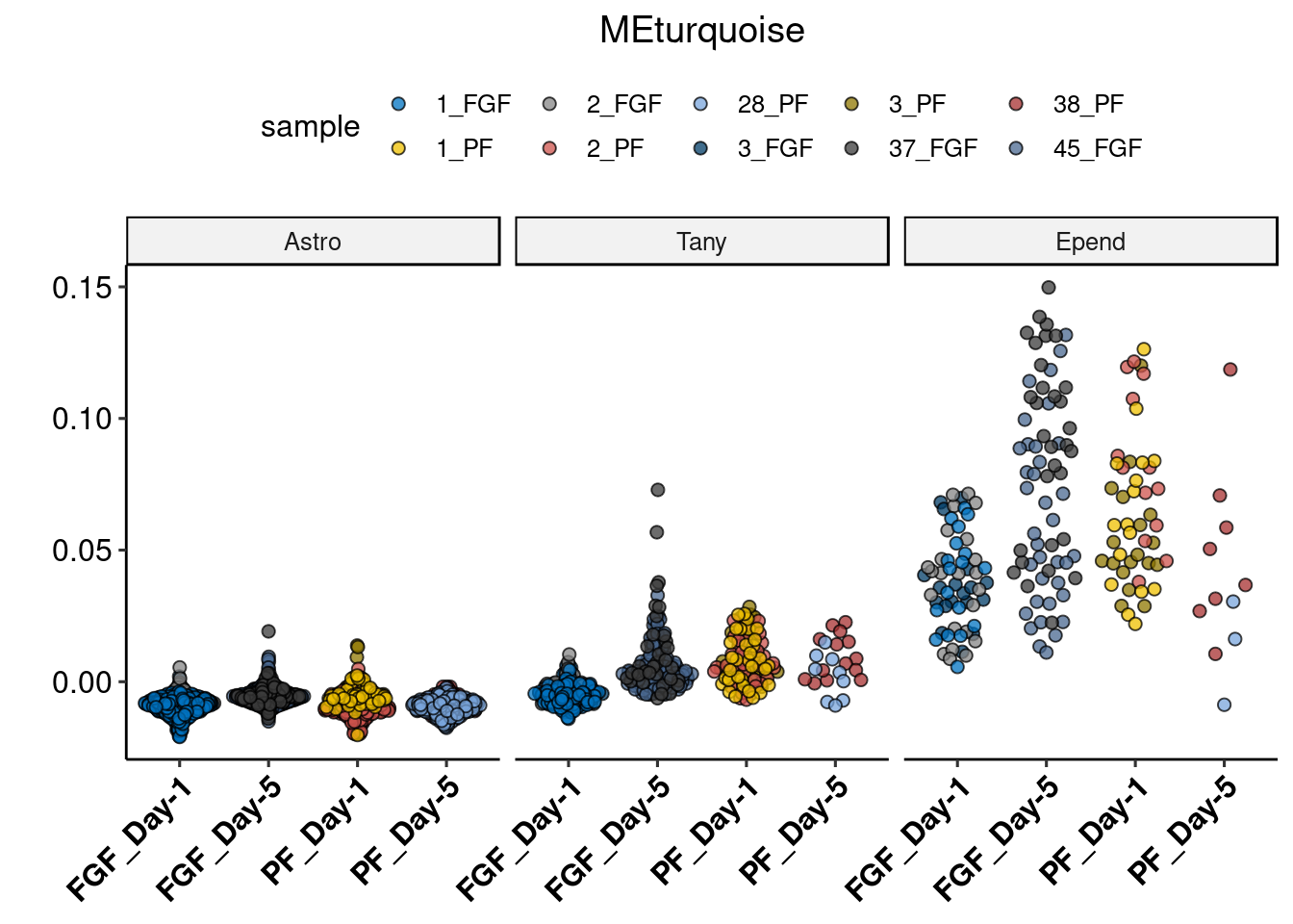
| Version | Author | Date |
|---|---|---|
| 9cf1e45 | Full Name | 2019-10-28 |
write_csv(sig, path=here("output/glia/wgcna/allglia_wgcna_linearmodel_testing.csv"))Plot change at D1 v change at D5 in each model per cell-type
sig %>%
unite(start, end, col = "comparison", remove = F) %>%
filter(comparison == "FGF_Day-1_PF_Day-1" | comparison == "FGF_Day-5_PF_Day-5") %>%
unite(estimate, p.value, sep = ",", col = "value") %>%
dcast(id + celltype ~ start, value.var = "value") %>%
separate(`FGF_Day-1`, into = c("estimate_1", "p.value_1"), sep = ",") %>%
separate(`FGF_Day-5`, into = c("estimate_5", "p.value_5"), sep = ",") %>%
mutate(id = gsub(id, pattern = "ME", replacement = "")) %>%
mutate(col = if_else(as.numeric(p.value_1) < 0.1 | as.numeric(p.value_5) < 0.1, true = id, false = "white")) %>%
mutate(sig = if_else(as.numeric(p.value_1) < 0.1 & as.numeric(p.value_5) < 0.1, true = "red",
false = if_else(as.numeric(p.value_1) < 0.1, true = "blue",
false = if_else(as.numeric(p.value_5) < 0.1, true = "black", false = "")
)
)) %>%
mutate(id = ifelse(col=="white", yes = NA, no = paste0("sn-glia-M", as.numeric(fct_relevel(as.factor(col), "white", after=Inf))))) -> plot
cols <- unique(plot$col)
names(cols) <- cols
multmod_plot <- ggplot(plot, aes(x = as.numeric(estimate_1), y = as.numeric(estimate_5))) +
geom_point(data = filter(plot, sig != ""), aes(shape = celltype), size = 4) +
scale_shape(name="Cell-Type") +
geom_mark_ellipse(data = plot %>% filter(sig == "blue", p.value_1 != 0.0230780280327769), color = "black", linetype = "dashed") +
geom_point(size = 5, color = "grey70", aes(shape = celltype)) +
geom_point(size = 4, aes(color = factor(id), shape = celltype)) +
coord_flip(clip="off") + geom_hline(yintercept = 0, linetype="dashed") +
scale_color_npg(name = "Modules", na.value="grey",
labels=c("sn-glia-M1","sn-glia-M2","sn-glia-M3","sn-glia-M4","sn-glia-M5","p>0.05")) +
geom_vline(xintercept = 0, linetype="dashed") +
annotate(geom = "curve", x = 0.045, y = 0.02, xend = 0.03, yend = 0.005, curvature = .3,
arrow = arrow(length = unit(2, "mm"))) +
annotate(geom = "label", x = 0.045, y = 0.0225, label = "Up at D1", hjust = "left", ) +
annotate(geom = "curve", x = -0.01, y = 0.03, xend = -0.025, yend = 0.035,curvature = .3,
arrow = arrow(length = unit(2, "mm"))) +
annotate(geom = "label", x = -0.005, y = 0.025, label = "Down at D1\n Up at D5", hjust = "left") +
annotate(geom = "curve", x = 0.01, y = 0.015, xend = -0.011, yend = 0.02, curvature = .3,
arrow = arrow(length = unit(2, "mm"))) +
annotate(geom = "label", x = 0.015, y = 0.01, label = "Up at D5", hjust = "left") +
annotate(geom = "curve", x = -0.02, y = -0.009, xend = -0.013, yend = 0.002, curvature = .3,
arrow = arrow(length = unit(2, "mm"))) +
annotate(geom = "label", x = -0.02, y = -0.02, label = "Down at D1", hjust = "left") +
theme_bw() +
xlab(expression(bold(Day1~beta))) +
ylab(expression(bold(Day5~beta))) +
guides(shape = guide_legend(override.aes = list(size=4),
title.theme = element_text(face="bold", size=8),
label.theme = element_text(face="bold", size=8)),
color = guide_legend(title.theme = element_text(size=8, face="bold"),
label.theme = element_text(face="bold", size=8))) +
theme_figure
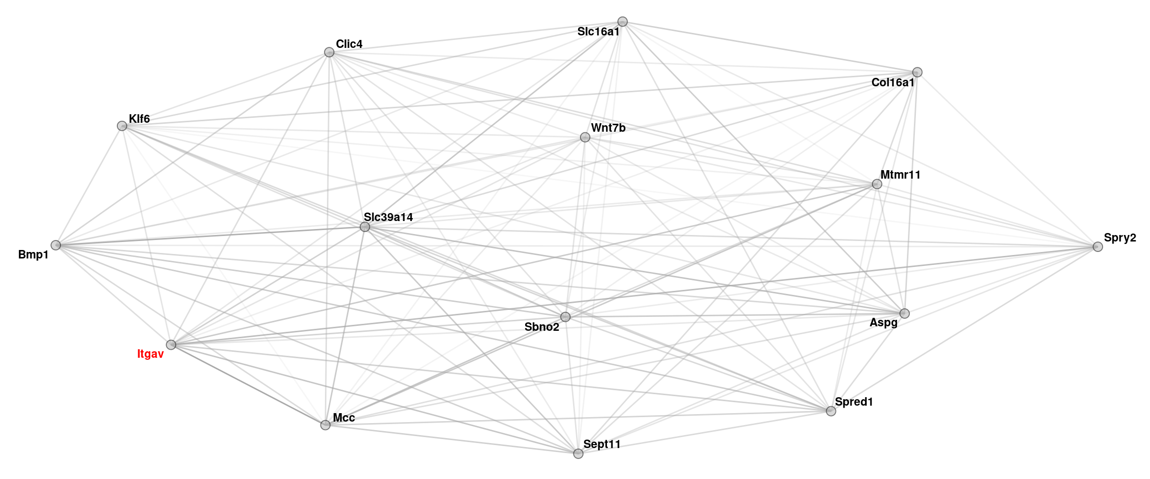
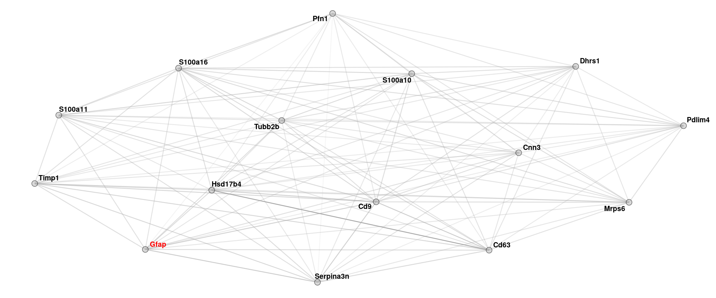
ggsave(here("data/figures/wgcna_res.png"), w=8, h=5)Plot gene networks
hubgenes <- lapply(seq_len(length(Network)), function(x) {
  dat <- modulekME[Network[[x]], ]
  dat <- dat[order(-dat[paste0("kME", names(Network)[x])]), ]
  gene <- data.frame(gene=rownames(dat),kme=dat[,x])
  return(gene)
})

names(hubgenes)<- names(Network)

color <- c("black","green","magenta")
lapply(color, function(col) {
  maxsize <- 15
  hubs <- data.frame(genes=hubgenes[[col]]$gene[1:maxsize], kme = hubgenes[[col]]$kme[1:maxsize], mod = rep(col,15))
}) -> hub_plot


hub_plot <- lapply(hub_plot, function(x) {
  adj[as.character(x$genes), as.character(x$genes)] %>%
  graph.adjacency(mode = "undirected", weighted = T, diag = FALSE) %>%
  as_tbl_graph(g1) %>% upgrade_graph() %>% activate(nodes) %>%
    dplyr::mutate(mod=x$mod) %>%
    dplyr::mutate(kme=x$kme)  %>%
    activate(edges) %>% dplyr::filter(weight>.15)}
)

hub_plot <- lapply(hub_plot, function(x) {
  x  %>%
    activate(nodes) %>%
    dplyr::mutate(color = ifelse(name %in% c("Gfap","Itgav","Vim","Sprr1a"), yes="red", no="black"))
})


set.seed("139")
plotlist <- lapply(hub_plot,  function(x) {
  print(ggraph(x,  layout = 'fr') +
  geom_edge_link(color="darkgrey", aes(alpha = weight), show.legend = F)  +
  scale_edge_width(range = c(0.2, 1)) + geom_node_text(aes(label = name, color=color), fontface="bold", size=3, repel = T) +
  geom_node_point(shape=21, alpha=0.5, fill="grey70", size=3) +
    scale_color_manual(values=c("gray0","red")) +
  theme_graph() + theme(legend.position = "none", plot.title = element_text(hjust=0.5, vjust=1), plot.margin = unit(c(0, 0, 0, 0), "cm")) + coord_cartesian(clip = "off"))
})
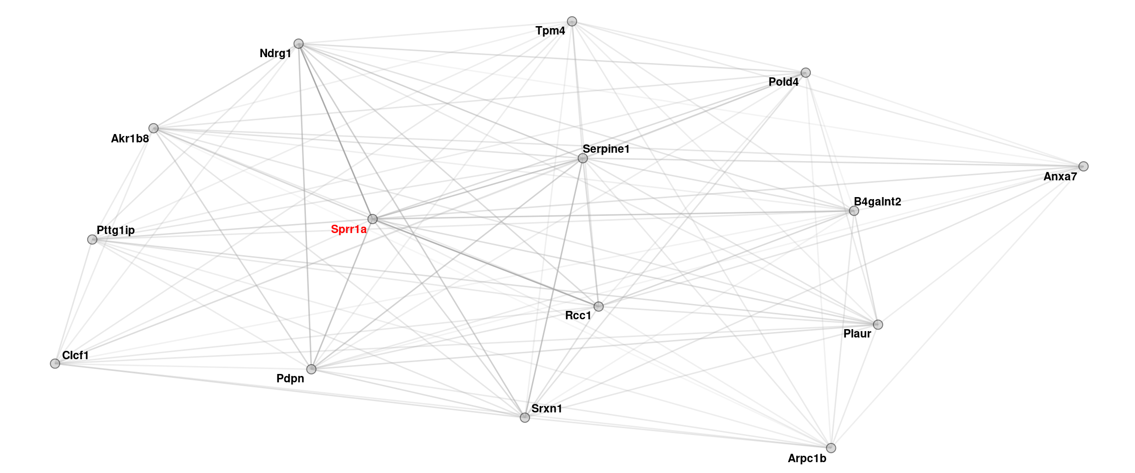
genenet <- plot_grid(plotlist[[1]], plotlist[[2]], plotlist[[3]], ncol=1, labels=c("f"), scale=0.9)load(here("data/figures/fig3/fig3_top.RData"))
fig_bot <- plot_grid(multmod_plot, genenet, nrow=1, align="hv", axis="tblr", labels=c("e",""), rel_widths =c(1.25,1), scale=c(0.9,1))
save(fig_bot, file = here("data/figures/fig3/fig3_bot.RData"))
fig_full <- plot_grid(fig3_top,fig_bot, ncol=1, rel_heights = c(1.5,1))
ggsave2(fig_full, filename = here("data/figures/fig3/fig3_arranged.tiff"), h=12, w=12, dpi = 600, compression="lzw")
fig_full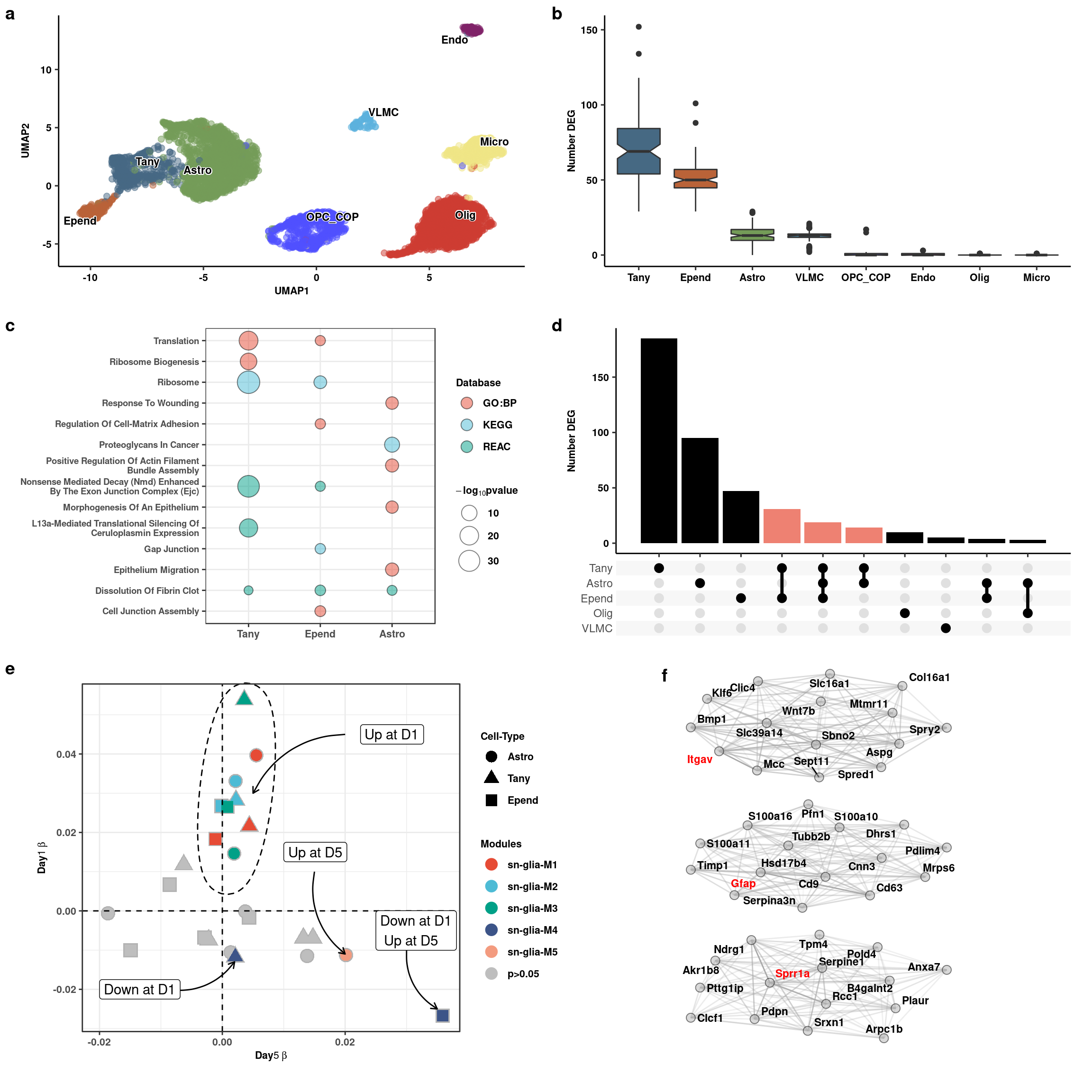
Find GO term enrichment of modules
go_col <- unique(plot$col)[-2]
goterms<-lapply(go_col, function(x) {
  gprofiler(as.character(hubgenes[[x]]$gene), ordered_query = T,
               organism = "mmusculus", significant = T, custom_bg = colnames(datExpr),
                           src_filter = c("GO:BP","REAC","KEGG"), hier_filtering = "strong",
                           min_isect_size = 3,
                           sort_by_structure = T,exclude_iea = T,
                           min_set_size = 10, max_set_size = 300,correction_method = "fdr") %>%
    arrange(p.value) -> got
  return(got)
})


names(goterms) <- go_col
goterms %>% bind_rows(.id="id") %>%
  mutate(padj=p.adjust(p.value, "fdr")) -> godat

write_csv(godat, path=here("output/glia/wgcna/allglia_wgcna_goterms.csv"))

godat %>% group_by(id) %>% filter(id %in% c("black","green")) %>% arrange(p.value) %>% slice(1:5) %>%
  select(p.value, padj, term.name, domain, id) %>% arrange(id) %>%
  ggplot(aes(x=str_wrap(term.name,20), y=-log10(padj), fill=domain)) + geom_col() +
  scale_fill_npg() +
  facet_wrap(.~id, scales="free_y", ncol=1) + theme_pubr() +
  theme(text = element_text(size=7),
        axis.text.x = element_text(angle=45, hjust=1)) + coord_flip() +
  xlab("GO Term") + geom_hline(yintercept = -log10(0.05), linetype="dashed", size=1) +
  labs_pubr()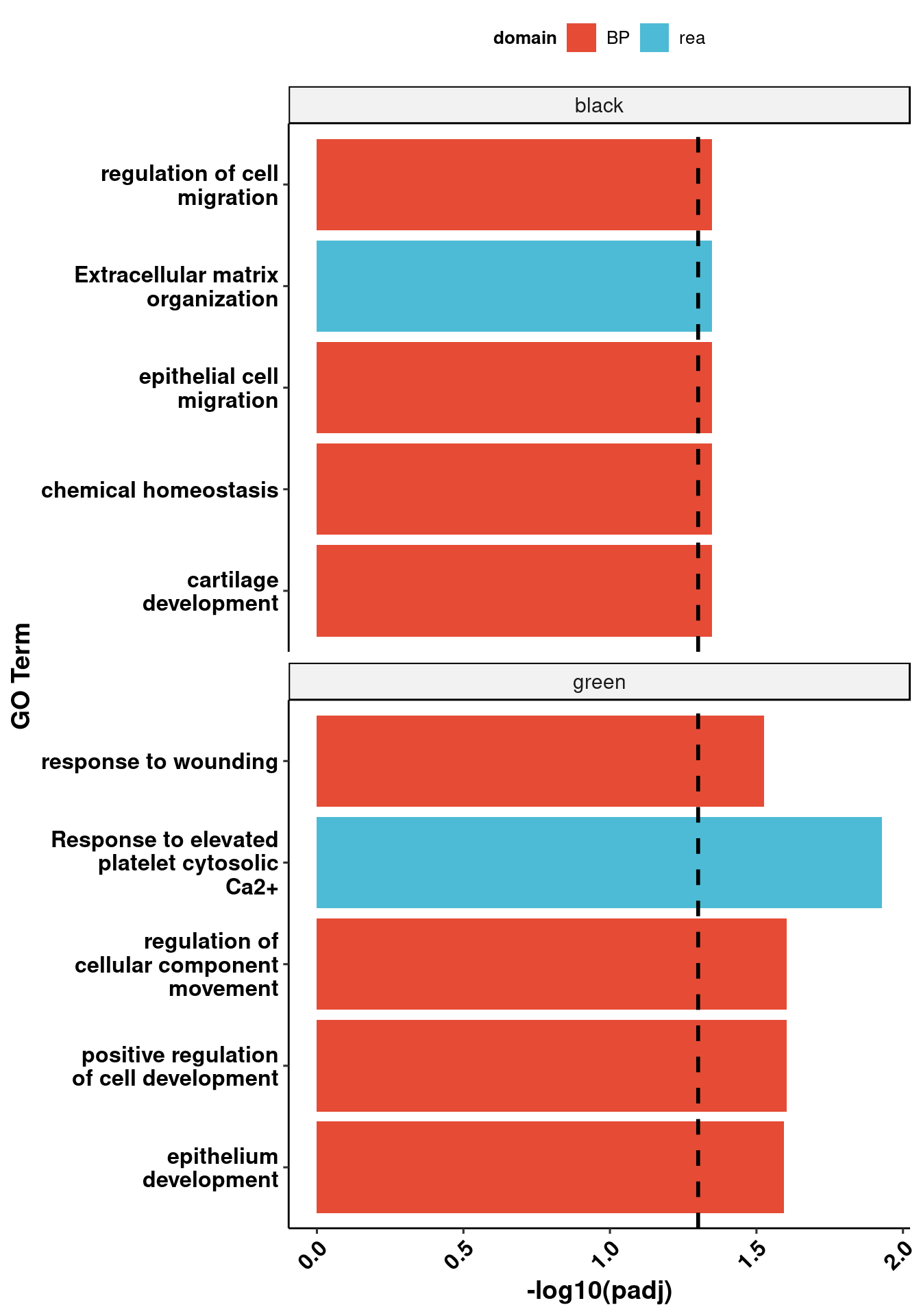
ggsave(filename = here("output/glia/wgcna/allglia_goterm.png"), h=6, w=8)
sessionInfo()R version 3.5.3 (2019-03-11)
Platform: x86_64-pc-linux-gnu (64-bit)
Running under: Storage
Matrix products: default
BLAS/LAPACK: /usr/lib64/libopenblas-r0.3.3.so
locale:
[1] LC_CTYPE=en_DK.UTF-8 LC_NUMERIC=C
[3] LC_TIME=en_DK.UTF-8 LC_COLLATE=en_DK.UTF-8
[5] LC_MONETARY=en_DK.UTF-8 LC_MESSAGES=en_DK.UTF-8
[7] LC_PAPER=en_DK.UTF-8 LC_NAME=C
[9] LC_ADDRESS=C LC_TELEPHONE=C
[11] LC_MEASUREMENT=en_DK.UTF-8 LC_IDENTIFICATION=C
attached base packages:
[1] stats graphics grDevices utils datasets methods base
other attached packages:
[1] future_1.14.0 cowplot_1.0.0 ggraph_1.0.2
[4] tidygraph_1.1.2 ggforce_0.3.0.9000 here_0.1
[7] ggpubr_0.2.1 magrittr_1.5 gProfileR_0.6.7
[10] igraph_1.2.4.1 reshape2_1.4.3 forcats_0.4.0
[13] stringr_1.4.0 dplyr_0.8.3 purrr_0.3.2
[16] readr_1.3.1.9000 tidyr_0.8.3 tibble_2.1.3
[19] tidyverse_1.2.1 genefilter_1.64.0 ggbeeswarm_0.6.0
[22] ggplot2_3.2.1 lme4_1.1-21 Matrix_1.2-17
[25] emmeans_1.3.5.1 ggsci_2.9 parallelDist_0.2.4
[28] cluster_2.1.0 WGCNA_1.68 fastcluster_1.1.25
[31] dynamicTreeCut_1.63-1 Seurat_3.0.3.9036
loaded via a namespace (and not attached):
[1] reticulate_1.13 R.utils_2.9.0 tidyselect_0.2.5
[4] robust_0.4-18.1 RSQLite_2.1.1 AnnotationDbi_1.44.0
[7] htmlwidgets_1.3 grid_3.5.3 Rtsne_0.15
[10] munsell_0.5.0 codetools_0.2-16 ica_1.0-2
[13] preprocessCore_1.44.0 withr_2.1.2 colorspace_1.4-1
[16] Biobase_2.42.0 highr_0.8 knitr_1.23
[19] rstudioapi_0.10 stats4_3.5.3 ROCR_1.0-7
[22] robustbase_0.93-5 ggsignif_0.5.0 gbRd_0.4-11
[25] listenv_0.7.0 labeling_0.3 Rdpack_0.11-0
[28] git2r_0.25.2 polyclip_1.10-0 farver_1.1.0
[31] bit64_0.9-7 rprojroot_1.3-2 vctrs_0.2.0
[34] coda_0.19-3 generics_0.0.2 TH.data_1.0-10
[37] xfun_0.8 R6_2.4.0 doParallel_1.0.14
[40] rsvd_1.0.2 bitops_1.0-6 assertthat_0.2.1
[43] SDMTools_1.1-221.1 scales_1.0.0 multcomp_1.4-10
[46] nnet_7.3-12 beeswarm_0.2.3 gtable_0.3.0
[49] npsurv_0.4-0 globals_0.12.4 sandwich_2.5-1
[52] workflowr_1.4.0 rlang_0.4.0 zeallot_0.1.0
[55] splines_3.5.3 lazyeval_0.2.2 acepack_1.4.1
[58] impute_1.56.0 broom_0.5.2 checkmate_1.9.4
[61] modelr_0.1.4 yaml_2.2.0 backports_1.1.4
[64] Hmisc_4.2-0 tools_3.5.3 gplots_3.0.1.1
[67] RColorBrewer_1.1-2 BiocGenerics_0.28.0 ggridges_0.5.1
[70] Rcpp_1.0.2 plyr_1.8.4 base64enc_0.1-3
[73] RCurl_1.95-4.12 rpart_4.1-15 viridis_0.5.1
[76] pbapply_1.4-1 S4Vectors_0.20.1 zoo_1.8-6
[79] haven_2.1.0 ggrepel_0.8.0.9000 fs_1.3.1
[82] data.table_1.12.2 lmtest_0.9-37 RANN_2.6.1
[85] mvtnorm_1.0-11 whisker_0.3-2 fitdistrplus_1.0-14
[88] matrixStats_0.54.0 hms_0.5.0 lsei_1.2-0
[91] evaluate_0.14 xtable_1.8-4 pbkrtest_0.4-7
[94] XML_3.98-1.20 readxl_1.3.1 IRanges_2.16.0
[97] gridExtra_2.3 compiler_3.5.3 KernSmooth_2.23-15
[100] crayon_1.3.4 minqa_1.2.4 R.oo_1.22.0
[103] htmltools_0.3.6 pcaPP_1.9-73 Formula_1.2-3
[106] rrcov_1.4-7 RcppParallel_4.4.3 lubridate_1.7.4
[109] DBI_1.0.0 tweenr_1.0.1 MASS_7.3-51.4
[112] boot_1.3-22 cli_1.1.0 R.methodsS3_1.7.1
[115] gdata_2.18.0 parallel_3.5.3 metap_1.1
[118] pkgconfig_2.0.2 fit.models_0.5-14 foreign_0.8-71
[121] plotly_4.9.0 xml2_1.2.0 foreach_1.4.4
[124] annotate_1.60.1 vipor_0.4.5 estimability_1.3
[127] rvest_0.3.4 bibtex_0.4.2 digest_0.6.20
[130] sctransform_0.2.0 RcppAnnoy_0.0.12 tsne_0.1-3
[133] cellranger_1.1.0 rmarkdown_1.13 leiden_0.3.1
[136] htmlTable_1.13.1 uwot_0.1.3 gtools_3.8.1
[139] nloptr_1.2.1 nlme_3.1-140 jsonlite_1.6
[142] viridisLite_0.3.0 pillar_1.4.2 lattice_0.20-38
[145] httr_1.4.1 DEoptimR_1.0-8 survival_2.44-1.1
[148] GO.db_3.7.0 glue_1.3.1 png_0.1-7
[151] iterators_1.0.10 bit_1.1-14 stringi_1.4.3
[154] blob_1.1.1 latticeExtra_0.6-28 caTools_1.17.1.2
[157] memoise_1.1.0 irlba_2.3.3 future.apply_1.3.0
[160] ape_5.3